Covid-19 thoughts / Formation of synthetic magnetite nanoparticles with peers

I think most people went through (and are still going through) a reflective period during this pandemic and times of isolation. We stayed home longer than ever before, deprived of day-to-day routines and activities, and were left to ponder our own value and individual purpose. Covid-19 is not an alien invasion, nor some other existential crisis, but a biological hazard that we will come to better understand how it infects, how to prevent its spreading, and potentially how to eradicate it. It is good to remember that these times are unprecedented and it is okay to have feelings of uncertainty. We are all in this together (not to quote Red Green…https://en.wikipedia.org/wiki/The_Red_Green_Show) and the best thing is to find ways to stay comfortable, relaxed and occupied, either with some work, new/old hobbies or anything you enjoy.

During confinement, I was in a fortunate position to be able to continue my work from home. I sifted through data that I had accumulated over the past two years, analyzing data and working up results. Through video conferencing it was possible to stay connected with others in the research group and to feel somewhat motivated and focused on work-related tasks. I will admit that working from home had some perks in the first few weeks, but after a couple of months it became a chore, trying to find ways to coax myself into work-mode. My level of motivation dipped and the line separating work from leisure became blurred. Alas, the conditions for working were far from normal so the expected amount of productivity should be scaled accordingly for anyone in the same position. Luckily, I was able to return to the lab in June and have been going steadily since. With the current second wave of cases and hospitalizations, who knows how long that will last.

Due to SARS-CoV-2, my last beamtimes scheduled for June and July were postponed until the late summer and early 2021. So, while my own measurements are on pause, I decided to write about a couple of beamtimes that I participated in as a colleague and collaborator over the last couple of years. One opportunity attached to research is the potential for collaboration and for sharing ideas and insights. Sometimes applying your knowledge and skills to a new set of problems outside of your own daily research tasks can lead to new perspectives and findings. I was grateful to be involved in two projects on the formation of synthetic magnetite (Fe₃O₄) nanoparticles, which used X-ray absorption fine structure spectroscopy (XAFS, how this technique works was previously described in the “Advanced Photon Source: …” post) to help understand nanoparticle growth mechanisms (how individual Fe ions come together to form small iron oxide clusters, and proceed to final larger Fe₃O₄ nanoparticles). These nanoparticles are essentially the same material produced by magnetotactic bacteria (the famous critters I have been talking about in previous posts), but they are instead formed purely by chemical means with no biology involved. Primarily, the synthetic magnetite nanoparticles examined in these works were of interest to understand fundamental processes governing formation and structure, but the materials themselves have application as catalytic materials, magnetic data storage devices and for biomedical application (hyperthermia treatment of cancerous tissue and magnetically-guided drug delivery, for example).

The first project and XAFS beamtime I will discuss was led by Dr. Lucas Kuhrts, a freshly minted PhD from the Max-Planck Institute for Colloids and Interfaces (MPICI, where my own post doc project began in 2018). Lucas had been studying the formation of magnetite nanoparticles with the addition of polymers (long, linear chains of repeated chemical groups), which changes the way smaller iron oxide clusters form larger nanoparticles. When I had first met Lucas, he had already performed a thorough investigation of the polymer-magnetite system with small angle X-ray scattering (SAXS), a technique that measures how incident X-ray light is scattered by particles in the sample, giving information on the size, density, and shape of those particles. In order to complete his formation mechanism, I suggested to assist in performing XAFS measurements to learn more about the local environment of iron atoms and the particular phase of iron oxide that may exist at various time-points in the synthesis. Upon agreement of applying XAFS to help solve his problem, we wrote a beamtime proposal and were awarded a few days at the Diamond Light Source in the UK (where I had already performed X-ray microscopy measurements, as shown in previous posts).

Fast-forward a few months after our awarded beamtime notice and here we were at the I-20 Scanning beamline of Diamond Light Source. Along with Lucas and I, was Oliver Späker, a PhD researcher also from MPICI. The important questions we wanted to answer regarding the formation of polymer-magnetite nanoparticles took place on a time-scale of minutes, where the crucial formation steps occur in the first minute to several tens of minutes after iron precursors, polymer, and base are added together for the chemical reaction and formation of magnetite, which proceeds as follows:

2FeCl_3(aq) + FeCl_2(aq) + 5NaOH_(aq) >>> Fe₃O_4(s) + 5NaCl_(aq)

You will see two different iron chloride salts for the reactants, which are the valence states of 2+ and 3+ needed to form the mixed valence that is magnetite (Fe(II)Fe(III)₂O₄). Considering the rate at which we could collect a single spectrum at I-20 Scanning for our dilute samples (low concentrations of Fe, with ~10-15 minutes per spectrum and several would need to be collected to improve signal to noise) and the several early time points we wanted to investigate, an in situ measurement was not feasible (this is where the measurements would be conducted on a sample environment where the chemistry is happening in real-time). This would mean that by the time we started and finished the collection of just one spectrum, the formation of magnetite nanoparticles would have been nearly complete. Therefore, we took an ex situ approach (the samples to be measured were taken from the natural sample conditions at various time-points and then preserved for later measurement). Here, samples were extracted from the chemical reaction at the time points of interest and were immediately frozen on a sample holder using liquid nitrogen.

Side profile of Lucas Kuhrts in the chemical laboratory preparing a series of polymer-stabilized magnetite nanoparticles

Filling the sample chamber with liquid nitrogen to keep the extracted samples frozen and also to improve the quality of the collected data.

The truly heroic aspect of this beamtime was that Lucas had brought his experimental apparatus with him from Berlin to Oxfordshire. Since we were not exactly sure which time points would be of most interest to capture the formation mechanism with XAFS (somewhere between 1-20 minutes…), Lucas would synthesize a series of samples, we would measure them, analyze the data to understand how iron oxide particles were forming and growing, and then redo it over again until we had samples at various time-points that gave us an overall picture of the chemical and physical process. It was a lot of work and determination on Lucas’s part, where Oliver and I tried to keep a broader view of the experiments and measurements to make sure we would have enough data by the end of the beamtime to complete Lucas’s study. In the end, we came away with information we had hoped to gain. We were able to capture how the added polymer affects the formation of magnetite nanoparticles: by delaying the rapid formation of magnetite phase by a precursor iron oxide phase known as ferrihydrite that interacts with the added polymer. We were so pleased with ourselves that we brought the news and the experimental apparatus to the Queen in London…

*Lucas and the titration apparatus used to produce magnetite nanoparticles* in front of Buckingham Palace

The second collaborative beamtime was also conducted at Diamond Light Source, at the sister beamline of I-20 Scanning, named I-20 Energy Dispersive EXAFS (I-20 EDE). The leader of this beamtime was Dr. Jens Baumgartner, a postdoctoral researcher at the time from MPICI. Joining him were myself and Lucas. Jens had been studying the formation of magnetite for several years since his PhD and has become well known in the field of biomineralization, examining magnetite formation from both biological and synthetic perspectives. One of the long-withstanding questions surrounding magnetite formation, and other many other minerals for that matter, is the exact nature of precursors that first form (nucleation) and directed the formation of the final nanoparticle product (growth). Capturing this chemical and physical information of nanoparticle growth at very early stages would provide an intimate understanding on how to better control inorganic nanocrystal growth, which would open up new approaches to design advanced nanomaterials. Again, very fundamental research objectives, but the principle is to enable more synthetic control over nanoparticle formation, which would have broad implications for future nanotechnology.

To capture information on the fast chemical and physical formation of magnetite we really needed to measure what is occurring on the time scale of seconds. More like milliseconds, actually… And for this reason Jens had chosen the I-20 EDE beamline to conduct this XAFS experiment. The EDE technique specializes in collecting an entire XAFS spectrum in a matter of milliseconds with even microsecond time scales feasible with today’s detector technology (whereas in the above beamtime, it took about 10 minutes for one spectrum). Generally speaking, we were able to collect an entire spectrum 60000 times faster than with the previous XAFS technique! Of course, there are some disadvantages with using such a fast technique. Mainly, the concentration of you material or element of interest has to be at higher concentrations. The concept of the energy-dispersive measurement is quite interesting. The following image shows the principle behind the measurement. The general idea is that one spectrum can be collected instantaneously, in a matter of milliseconds, which is highly advantageous for capturing fast chemical formation processes.

Energy Dispersive EXAFS - - Diamond Light Source — Energy-dispersive EXAFS concept. Instead of a monochromatic X-ray beam scanned across the absorption edge (standard XAFS, which can take a few minutes), a dispersed polychromatic X-ray beam is created by diffraction off of a curved crystal, which is then focused on the sample position (note how the different X-ray energies (colours, here) converge on the sample and then diverge toward the detector). The energies of the polychromatic X-ray beam are tuned to cover the X-ray absorption region of the element of interest (iron….as always). The detector then collects the X-ray beam intensity over a large number of camera pixels to bin each energy position. Together this creates a single XAFS spectrum in one X-ray flash.
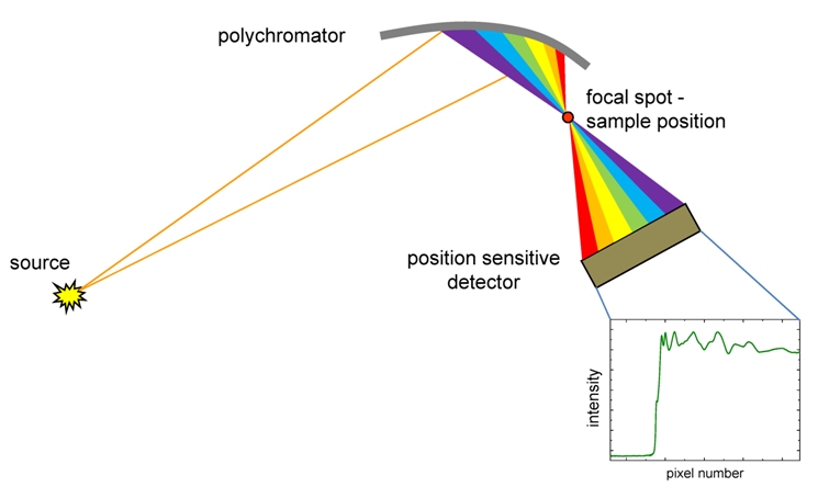
Image source: https://www.diamond.ac.uk/Instruments/Spectroscopy/Techniques/EDE.html

So with a fast method of collecting data, how to trigger the chemical reaction in a controlled and precise manner? For this a stopped-flow device was used, which can be seen in the images below. There, several plastic syringes can be seen installed into a stainless steel block and are controlled by a pressurized pump. On top and in the middle of this block is where solutions from the syringes are injected and subsequently mixed, contained inside a thin X-ray transparent tube (i.e., a capillary of Kapton polymer). As the solutions come in contact with one another in this tube, the formation of magnetite proceeds. It is also the exact position where the dispersed X-ray beam converges and then diverges toward the detector. The stopped-flow device is specially designed for the study of fast chemical processes because it can deliver highly accurate volumes of each solution into the measurement region and with coordinated precision to ensure the reaction will proceed in the same manner each repetition. The triggering mechanism can be controlled remotely, as we did this when we were safely outside of the experimental beamline hutch and in the control room. This way, we could trigger the reaction and start the XAFS measurement simultaneously.

Lucas and Jens running first tests on the stopped-flow device to ensure each solution is being triggered correctly.

This beamtime was technically challenging. Also, an exhausting for the team since we had to enter the experimental hutch to recharge the solutions and make any minor adjustments to the stopped-flow device. One of the first things needed to be done was to determine the right concentration of Fe to use in the solutions. If the concentration was high, there was a good XAFS signal, but the formation of magnetite occurred too fast to capture. If the concentration was low, the X-ray absorption on the sample would be too weak, resulting in XAFS data that was too noisy to work with. After finding the right concentration, more problems would arise and it was a struggle to keep things going enough to collect meaningful data to complete a study. But thanks to a lot of coffee and several days of beamtime, things came together and we left with a lot of data… A LOT. I do not have the definitive numbers in front of me but we were collecting about 50000 spectra every 5-10 minutes and we had about 7 days of beamtime. Needless to calculate, we left with millions of spectra on the formation of magnetite! There are definitely some exciting things to come from the analysis of this data (from both beamtimes).

I look forward to sharing the next synchrotron trips and adventures with you, but I am not quite sure when that will be exactly. I had conducted a recent beamtime remotely from home, which was a great experience and could be the temporary future of synchrotron measurements… Anyway, we will see and I will update again soon with other synchrotron trips and recent events that I have yet to share. Until then, take care and wash your hands.

X-ray data hangover / “Here comes the sun”: first trip to Soleil synchrotron

I have recently finished up several beamtimes and attempting here to summarize all of the recent going-ons related to my research. Since my last post (in November! oops) I have traveled back to ALBA (Barcelona) for more X-ray tomography measurements (December), went to Soleil synchrotron (Paris) twice (December and February) for my first measurements with scanning transmission X-ray microscopy and returned to Diamond (Oxfordshire, UK) for a final round of X-ray nanoprobe tests (January).

…phewfff…

All in all, each beamtime went well, with about 9-10 terabytes of data collected in total. This amount of data is on a scale I haven’t dealt with before. The need to constantly purchase external hard drives is something that I did not anticipate. Luckily the price for data storage is quite affordable these days.

“Data overload. All USB ports are busy at the moment.”
Recent beamtimes have filled three more large external hard drives.

X-ray tomography (essentially a 3D reconstruction of the sample from 2D X-ray images) efforts at ALBA were dedicated to my colleague Yeseul’s PhD research, which is on a sulfate-reducing magnetotactic bacteria that is known to produce iron sufides in addition to iron oxides. We had run a few tests during the previous beamtime in July, but the bacteria were experiencing severe radiation damage due to the high amount of heavier elements (e.g., sulfur, iron and other metals) in this type of bacteria, which were absorbing a lot of the incoming X-rays. In anticipation of this issue, which my samples did not experience as drastically before, we had prepared samples with a thicker layer of ice to reduce the amount of X-rays absorbed by the bacteria. However, by reducing the dose of X-rays on the bacteria, a reduction in image resolution resulted. In the end we were able to come away with a few tomograms to understand a bit more about the magnetotactic bacteria, particularly what the bacteria seem to be producing inside their cell body. So overall, it was a success.

Standing above the control room of the MISTRAL beamline. This view shows how the experimental station (below, near red crane) branches off the electron storage ring. This image was taken during a late night synchrotron stroll in an effort to stay awake while working late.

Yeseul in control at the MISTRAL beamline. It took several attempts to find cells to measure that were covered in just the right amount of ice to prevent radiation damage during an X-ray tomography scan.

Shortly after returning from ALBA by car I headed to Soleil synchrotron a few days later… also by car. Going by car was not intended but due to transit worker strikes in France and the general dissatisfaction with the latest pension reform in France, our trains were cancelled. I have to thank my PI and fellow post doc Matthieu Amor for joining me on this journey and providing their driving services. After the northern voyage across central France we set up shop at the scanning transmission X-ray microscopy (known as the STXM technique) beamline HERMES to take measurements on single magnetotactic bacteria dried on substrates and in a liquid cell. The latter measurements were the main challenge and objective of the beamtime: “is it possible to measure a single bacterium in liquid and be able to resolve the internal biomineral structures within?” From preliminary tests, we were able to achieve enough contrast between the cell membrane and the surrounding water in order to image the bacterium. However, the water layer was still too thick (on the order of a few tens of microns) so it was more difficult for softer X-rays to penetrate the entire sample and liquid cell and then be detected.

These liquid cell tests are different from the ones I had performed at the hard X-ray nanoprobe at Diamond because soft energy X-rays are used for STXM. With lower energy X-rays, there is less penetration of X-rays through matter (in other words, substances like silica, water, organic material absorb a higher percentage of incident X-rays leaving less radiation to pass through the sample and reach the detector behind the sample (see below for experimental setup). So why use softer X-rays if it introduces more limitations to measuring bacteria in water? One main advantage is that the X-ray beam size is even smaller for STXM (~20-30 nm) than for hard X-ray nanoprobes (~50-100 nm) and lighter elements such as those from the cell membrane and other intracellular components (C, N, O, P) can be measured in addition to the iron oxide biominerals contained in the cell. If we can manage to observe these organisms on such a scale while also still living (or near their native-cell state), a whole new level of intracellular information can be captured in real-time. Particular to the X-ray techniques that I am using, information on the role of metals in nanoparticle formation within microorganisms is hoped to be achieved.

Pictures below show the STXM beamline at Soleil synchrotron and the sample environment with some features labelled. The sample environment is quite cramped, mainly because of the reason I mentioned above: softer X-rays are absorbed or scattered more easily by gas molecules and condensed matter, so the delivered X-rays from the synchrotron must pass through the lens, the aperature, the sample and then the detector. The greatest challenge with imaging bacteria in water with soft X-rays is the thickness of the water layer. This cannot exceed a few mircons otherwise the percentage of X-rays that can pass through the liquid cell will be too low to be used to discern any contrast between the bacteria and the background. Our tests this time were to rerun the tests with the liquid cell and to use a spacer material that was around 0.5 to 1 mircon (10E-6 meters). This incredibly small spacing is used between the two windows of the liquid cell to determine the water thickness.

The HERMES beamline in Soleil Synchrotron (Paris, France). HERMES is a scanning transmission X-ray microscopy beamline. It uses a tiny beam size of 20-30 nm of soft energy X-rays and a sample stage that moves the sample of interest over this beam. In the picture, the X-ray beam is delivered from the left side (through the evacuated tubing covered in aluminum foil) and enters the large vacuum chamber seen in the middle. An evacuated chamber is necessary since lower energy X-rays are more easily absorbed by gas molecules than higher energy X-rays.

Here is an image from within the vacuum chamber (shown above). Indeed, things are cramped in here. The distance from the focusing lens to the detector is only a few millimeters, so the installation of samples and the sample thickness requirements are restricted. Since this is a transmission measurement, it is easy to understand how an image is collected. The X-rays are focused onto the position where the sample is expected to be to achieve minimum beam size. The sample is scanned over the beam position (motorized stage below the sample plate). Lastly, the detector (photomultiplier device – converts detected photons into an electric current) detects the change in transmitted X-rays, which will distinguish pixels (or regions) of the sample that are more electron dense than others or where the absorbing element of interest is located (for me, it’s iron, of course!).

An example of what a STXM image (2D map) looks like for a magnetotactic bacterium. This image was collected at 715 eV, the energy at which Fe will more strongly absorb over other metals. As a result, the iron oxide nanoparticle chain can be seen clearly against the background and the cellular membrane. Each pixel is 25 nm.

This is the liquid cell set-up that was tested at HERMES. It is a device similar to what is found for measuring liquids for electron microscopy, but with a few modifications to suit the STXM beamline. Needless to say, we were unable to get the successful result that we were hoping for, but we are planning again for another chance!

Working next to the beamline scientist in charge during my beamtime, Dr. Sufal Swaraj. He showed a great deal of dedication in helping me with my first round of measurements. The liquid cell tests are very time consuming (each attempt requires 3-4 hours of set-up, all going well). With his continued support, my hopes are high that we will get closer to my (but also, our) goal of measuring more bacteria in liquid.

After accumulating plenty of data over the last three months and realizing that there are several tasks that are to be tackled in the next few months, things are getting busy… very busy. At this stage of my post doc position, I only have about 7 months left in my contract. I not only have to start writing up papers on what I have accomplished thus far, I have to start looking for a new research position. This involves writing applications, proposals, cover letters and going for interviews. And with the recent COVID-19 outbreak, some of these tasks will be challenging to accomplish (especially travel-related ones). Luckily, I do not have any synchrotron trips until June/July, so hopefully things will return to normal by then…
Hopefully!

Communicating research and a second chance at the Diamond X-ray nanoprobe

European Night of Researchers

The last month was full of preparations for October’s upcoming measurements at Diamond Light Source, but it also included my involvement as a participant in the “European Night of Researchers”. The event is hosted across several European countries on the same evening for the general public. Check out these links for more info:
https://nuitdeschercheurs-france.eu/?EntrezdanslEnquete and https://ec.europa.eu/research/mariecurieactions/actions/european-researchers-night_en The event is a great chance for those interested in science and technology to have a conversation with people conducting research on topics or issues that may not be well known to most. I participated in the event held in Marseille to discuss with people of all ages and backgrounds in short 10 minute one-on-one discussions about my research. It is often challenging to sum up what a researcher does on a day to day basis and to communicate the importance or relevance of their work. One approach of the evening was for the researcher to bring an object with them that could create some discussion about the work and to spark some curiosity. I attempted to do this by bringing along a small culture of magnetotactic bacteria and a magnet to control the bacteria from the outside. By shining my cell phone light into the test tube, scattering of the light would change direction when I moved the magnetic field to manipulate the bacteria. Check out the link below for a quick demo. It was a simple demonstration to reveal the peculiar ability of the bacteria, which created opportunities to discuss directly on this property. From this demonstration, conversations led to exploring the idea of the bacteria utilizing the magnetic field of the earth to locate preferential metabolism conditions, how humans could manipulate them for biomedical technology and thus, why we are interested in understanding the mechanism for forming such magnetic nanoparticles within the cell. The consensus seemed to be intrigue and surprise – people seemed fascinated – so, mission successful.

Magnetic control over bacteria Download

A snapshot of “Into the Survey” during European Night of Researchers in Marseille, France (September 2019)

The only thing that time did not allow for was to go into more detail on what kind of experiments/techniques I use. It is often difficult for researchers to explain what they do with simple terms and it is something they have to work on. There are some research projects that can be easily summed up in a couple of sentences using non-jargon words. Whenever the topic of synchrotrons or using X-rays for my projects comes up in conversation, this gives rise to another aspect of my research that demands further explanation. I struggled with this for some years during my PhD where I didn’t want to dumb down or oversimplify what I was doing for research, but also did not want to over complicate the explanation of my activities (confusing the once interested, innocent bystander). An explanation of my PhD research ranged from “I investigate small luminescent gold particles that could be used for biomedical imaging and cancer detection applications” to more specific and technical, “I utilize X-ray absorption spectroscopy to study the electronic and structural properties of gold nanoclusters for an understanding of structure-property relationships”. The second is more accurate, but the first involves an application that people can imagine and see tangible motivation for the research. I have found over time that knowing your audience, how much time you have to explain and relating the research to commonly known things (e.g., batteries, MRI imaging,) can help make the interaction more efficient and enriching for both parties. For my topic of research anyway, I cannot rely on one or two sentences to give every time, a small amount of energy is given to tailor the level of detail and depth, while still keeping the overall objective consistent. It is still something I have to work on, but the effort is worthwhile so that more people can learn more about what’s going on in the modern world of science and technology.

A second round at Diamond using the X-ray nanoprobe

Back to the research, plenty of time was spent in September preparing microfluidic devices for measurement at the synchrotron. These devices, which contain the bacteria in micrometer-sized channels for X-ray measurement, still need some adjustments and modifications. There is only so much that I can prepare before these devices are used in front of the X-ray beam for a four-day experiment, which is valuable, valuable time (and goes by quickly)! Such tools are various optical and fluorescence microscopes available in my home institute. These tests give an indication for how the bacteria are doing in the microfluidic device (if the bacteria are immobilized in the device) and if the device is functioning properly (no leaking, consistent flow of liquid through the device). During these preparations for beamtime, I traveled back to the Max Planck Institute in Potsdam to prepare devices with a new microchannel design. I was fortunate to prepare these new devices with only one week before heading to the synchrotron (phewf!)

A dust-free working space for the preparing of clean microfluidic devices. On the left is a spincoater to create a thin layer of polymer material on a mold. On the right is a plasma cleaner, which is used to clean surfaces and make them more hydrophilic using a plasma of oxygen. This not only cleans the surface but also enable physical bonding of materials for the assembly of microfluidic devices. In the middle you see some of the assembled devices which are a support material bonded with a polymer layer. Again, I apologize that details are left out until the work is published.

So with updated microfluidic devices in hand and a few extra samples of magnetotactic bacteria to measure dry (not in liquid cell), I headed to Diamond. Similar to last trip, I brought with my trusty team of Elisa and Yeseul for lab and moral support. Again, measurements were conducted at the X-ray nanoprobe (see two posts ago for images and description of the location and technique) with the goal to measure the intracellular Fe content of magnetotactic bacteria at different stages of magnetosome growth (magnetite nanoparticle formation). Some of the beamtime was also dedicated to investigating Yeseul’s project of magnetotactic bacteria that produce iron sulfide nanoparticles instead of the iron oxide ones I study. She brought some dried samples to measure the intracellular iron and sulfur content to get an idea of the elemental distribution in each cell and the signal strength so that she can better prepare for her own beamtime in the future. The image below shows some of the struggle when trying to find a specific cell to measure. Yeseul had taken TEM images of her cells before measuring at the nanoprobe so there were certain cells to revisit. If there are no obvious reference points on your sample substrate (TEM grid), it takes a bit of skill to orientate yourself and the X-ray to find a 3 micron cell on a 3 millimeter grid!

I would have to say that the measurements with the microfluidic devices did not produce the final result I was hoping for this beamtime, which is to see the evolution of Fe X-ray fluorescence over time as magnetite is formed in each cell. The beamtime still served to verify and confirm a few things regarding how to operate the designed microfluidic devices in the beam, what limitations we have for measuring the Fe signal from individual cells and how long-term measurements of 6-8 hours should be conducted. Needless to say this project has been taking much longer than anticipated to get to the point where I can present something completed for publication or conference. The amount of skills and information I have learned of course has been valuable, but I am hoping the next series of measurements will be enough to settle on enough data and progress worth sharing with the scientific community.

The never ending war on microfluidic tubing, which runs from a syringe pump (containing media for the bacteria) to the microfluidic device (mounted in the X-ray beam) and then to waste (expelled media).

Overall, the four days of X-ray nanoprobe beamtime was utilized well. In addition to several tests with the microfluidic devices I had several dry samples of bacteria and algae (in collaboration) to measure for 2D mapping of metal distribution with 50 nm resolution. There is plenty to improve on for the next round so I better go and get started! … As a last note, I had also spent four days back at Diamond later in October with fellow synchrotroner, Lucas Kuhrts, helping him with X-ray absorption spectroscopy measurements (the same technique I used a few posts back at the Advanced Photon Source outside of Chicago, IL) relating to his own research on abiogenic magnetite formation (whereas my project is on biogenic magnetite formation). I plan to recap some of these additional synchrotron adventures outside of my own project in a later post.

Coming up next are trips to Soleil synchrotron (outside of Paris) and back to ALBA synchrotron (back to Barcelona), which are both in December and both are using low energy X-rays for microscopy purposes. Plenty to do before the end of this decade! Wish me luck. I hope to update soon.

A bientôt !

Tips for writing a beamtime proposal

Featured image of the ESRF facility (Grenoble, France)
(source: https://www.francetvinfo.fr/culture/patrimoine/le-synchrotron-de-grenoble-revolutionne-la-paleontologie_3288529.html)

Since the beamtime at Diamond for X-ray nanoprobe measurements (April-May) I have only had a short beamtime back at ALBA in July. I will wait to report on this research trip for my next post, where I will combine the details of the synchrotron trip with some other going-ons back at home base, CEA Cadarache. It has also been summer holidays in France. So trying to fully adapt to French life, I have been relatively inactive during the month of August. Don’t worry, there is plenty of synchrotron science in store for the fall and winter… I will be participating in over 400 hours of awarded beamtime at three different facilities! This is rather exciting, but daunting nonetheless. To make the most of the precious beamtime, there are many technical details that have to be considered for each measurement (experimental setup, X-ray technique and sample type). I hope to capture what these preparations (and the madness) entail in the next post. Here and now, I want to quickly discuss how synchrotron beamtime is awarded and what is required to write a competitive proposal to receive experiment time at a facility near you.

Every year there are two to three calls for beamtime proposals to be submitted with one of those calls coming up in September/October for many synchrotrons around the world (so this post could be timely for those interested…). If you are reading this as a graduate student who has an idea for a measurement that would highly benefit their project’s progress and must be performed using light from synchrotron radiation, please read on! Acquiring beamtime, though it is still highly competitive in some fields, is more possible than you think. The reader should be cautioned that there are various application processes depending on the synchrotron and several possible techniques for proposals to be written on. Along with the general experimental proposal covering background, research objective, methodology and expected outcomes, there are numerous details to be entered into the application. I am sharing some general pointers to get an experimental proposal started, but the requirements for each synchrotron and proposal type should be carefully read and considered.

What is beamtime?

Beamtime is allocated experimental time at synchrotron facilities and is mainly dedicated to researchers coming from academic research institutions. A smaller amount experimental time is available for industrial groups and they must pay a hefty price (~10-20k EUR per beamtime!). The beamtime for academic users is essentially free once awarded based on the submitted experimental proposal. The user will have to pay for remaining expenses such as travel, shipment of samples and equipment, and accommodation (although some synchrotrons provide additional funding for such costs). As can be imagined there is an immense amount of funding from government institutions and research partners each year to keep the synchrotron functioning properly and to provide beamtime to these eager researchers.

Choosing the technique

See here a quick, general overview of synchrotron-based techniques:
https://lightsources.org/about-2/techniques/

First off, determine the spectroscopy, microscopy or scattering technique(s) that is most suitable to answer the scientific question in mind. The chosen technique may be one that the prospective user is already familiar with and has available at their home institute, but access is requested at the synchrotron to obtain faster measurements, utilize a brighter light source, achieve better energy resolution or require more sensitive detection equipment. Most of the time researchers apply for a technique that they do not have regular access to and would benefit from outside of their routine analytical methods. To further aid in determining the correct technique for the experiment, check publications in databases within the research area including tags of X-ray, synchrotron, etc.; it could be that other groups have already used synchrotron-based techniques to solve a problem similar to one be detailed in the proposal. Also check the publications on the website for the beamline of interest. There could have been measurements performed already at the beamline that relate to the proposed experiment. Once a technique is chosen and an idea for what kind of measurements are to be conducted and on what kinds of samples, the best thing to do next is to make contact with a scientist at the beamline. If this is the first proposal or if the measurements proposed are not routine (X-ray diffraction of protein crystals would be considered routine), the prospective user will benefit immensely from this early exchange and it will improve the chances that the proposal will be considered and further, accepted. One reason is that technical details overlooked in the proposal could render your measurements impossible at the given beamline. Another possibility is the beamline operating conditions may have changed recently and the beamline’s website may not have been updated (…this may have happened to me…). All of the above should be done at least one month before the submission deadline to allow enough time for a few exchanges between the user and the beamline scientist, and if the beamline scientist is willing and interested, they may even provide quick feedback on the proposal (not every scientist will have time to do this, but it can happen).

Preliminary data

To strengthen the proposal, consider adding preliminary data that describes the sample or system under investigation. Ideally, previously acquired some preliminary data using the proposed technique can be used to demonstrate that the experiment is feasible and that the user understands how the data is acquired and handled, and how it can it is useful to answer the proposed scientific question. If no such preliminary data has been acquired using the synchrotron-based technique, it is possible to contact a beamline scientist to see if they would be able to run a test measurement. Of course this request should be made a few months in advance since the beamline scientist will have to receive the sample and then perform the measurement on one of the very limited days they have to run these test measurements. Preliminary data can also include other measurements that have already been performed on the sample or system for characterization. Even better, if these characterizations clearly show that the sample of interest is well characterized, but is lacking a deeper understanding of some aspect that can only be achieved using the desired synchrotron-based technique, this is perfect to use in the proposal.

How much beamtime time?

Every beamtime proposal requires an estimation for the number of shifts (typically 8 h per shift) or amount of time needed to complete the measurements for the designed experiment. While some applicants may throw in a value last minute before submitting, this is another important consideration for the justification of beamtime being awarded and to demonstrate that you understand all that is required for a complete experiment from start to finish. Often the proposal submission form will ask the user to explain how much time will be dedicated to specific tasks such as measuring standards, loading samples into cryo conditions, general measurement run times and the number of total samples or measurements to be completed. Again, if this is the first proposal and a new technique, the best option is to contact the beamline scientist for a proper estimation of beamtime needed. They usually provide a general estimation based on the quality of data you hope to acquire and the concentration and/or condition of your samples.

Selection committee

Since proposals are graded similar to peer-reviewed manuscripts, the selection committee and field of research should be chosen carefully. Even though the proposal should include a brief introduction to the field and background related to the experiments at hand, it is desirable that reviewers will already have a general understanding of how the findings will contribute or advance the research area. If they can foresee the impact from the beamtime, this will only increase the probability that it will be accepted. The other consideration for carefully selecting the committee is if your project is highly multidisciplinary, for example it involves a combination of sample types or techniques that are not common to one specific area of research. For example, I am conducting measurements on iron oxide nanoparticle formation within bacteria, which essentially combines research domains of chemistry, physics and biology. Because of this diversity, my project and proposals sometimes fit into to more than one reviewing panel. My advice, again, is to discuss with the beamline scientist. They might have some experience with proposals similar to the work proposed and can recommend a selection panel that will yield a greater chance of being accepted.

I hope these general tips and guidelines will shed some light (pun intended) on the process of beamtime applications. For those researchers applying in the near future for the first time, best of luck and feel free to contact me for more information.

Ciao ciao

Diamond beamtimes are not forever (working title, actual title)

Another beamtime, another synchrotron! This time I headed to the Diamond Light Source, which is situated within the Harwell Science Campus in the Oxfordshire region of the UK. Although it is exciting to go to a new synchrotron, this is not the most efficient practice. The reason for this trip was to utilize an X-ray technique that was new to me, to my project and to most of my group members. I would say that my project is still going through the testing phase where there are plenty of growing pains. Mainly, I am exploring different X-ray microscopy/spectroscopy techniques to find the beamline that will be most suitable for my research on magnetotactic bacteria and with the particular goal of capturing magnetosome growth in situ.

The impressive nanoprobe technique

This beamtime at Diamond was at the X-ray nanoprobe beamline (I-14), which provides X-ray beams of less than 100 nm in width within the hard energy range (4-30 keV) and can perform X-ray fluorescence mapping (creates a 2D map of a bacterium with the distribution of elements, such as iron, sulfur, phosphorus, etc.) and X-ray absorption spectroscopy (electronic and chemical state of element of interest, as discussed in previous posts). From the name “nanoprobe” it almost speaks for itself. The design and purpose of this beamline is to probe the structure and chemical nature of samples ranging from cells to rocks to metal alloys on the nanoscale. For my intended studies on nanoparticle formation within magnetotactic bacteria, this was an obvious choice for an X-ray technique that could provide the size resolution and the intense X-ray intensity to measure the formation of nano-size iron particles. One cool thing about this beamline is that it had to be constructed almost 200 m outside of the actual synchrotron in order to achieve such a nanoscale beam size! This is done through a series of long stretches of vacuum tubing, mirrors and slits. It is impressive that X-rays can be controlled to zap a single nanoparticle for structural/chemical information or even a single organelle of a cell.

Location of I14 nanoprobe outside of synchrotron https://www.wayforlight.eu/en/facility/22091
The I14 Nanoprobe beamline entrance on a lovely, early english morning

Getting to the actual measurements

Once the X-ray beam is focused to its nanosized dimensions, the actual measurement is straightforward. The sample is moved with fine motor control from side to side, up and down to allow the X-ray beam (which is stationary) to scan over the entire region of interest. In front of the sample and off to the side, there are X-ray fluorescence detectors which capture X-ray emission from the elements contained in the sample and this signal is plotted over a 2D special grid to indicate areas of element concentration. From this description you can see that even though this is another X-ray microscopy technique (in addition to the soft X-ray transmission microscope in my ALBA post), this method offers a completely different approach and different set of data to collect. Another significant advantage of the X-ray nanoprobe is the hard X-ray energies that can be achieved. This is particularly important for the main goal of measuring magnetotactic bacteria in liquid. The higher energy X-rays allows deep penetration through materials such as polymers, glass, water, cellular material so that the material of interest (iron oxide nanoparticles) can be measured with adequate collected signal. In comparison, if soft X-rays are used (~200 to 2000 eV), the X-ray intensity will drop drastically after they pass through a few microns of the materials mentioned above. Nevertheless, there is a balance between many of these X-ray microscopy techniques – one being the size of the X-ray beam and hence the size resolution. Soft X-ray microscopy techniques have achieved beam sizes on the order of 20-30 nm, which would be more comparable to the size of the magnetosome of magnetotactic bacteria, however the penetration depth is much lower.

For this beamtime, my experiments were divided into two trips so that the first beamtime could be used to learn the in’s and out’s of how to run experiments. First up was to test a range of samples to determine the range of chemical and spatial sensitivity for probing magnetosome formation in magnetotactic bacteria. To do this, I prepared a series of magnetotactic bacteria at various stages of magnetosome growth which were dried on TEM grids (copper metal mesh with 10 nm thick carbon film). An example of what the 2D X-ray fluorescence mapping data looks like is shown below. With the X-ray beam being 100 nm, the TEM grid (with bacteria deposited) is scanned side to side and up and down in front of the beam. First starting with large steps of 1000 nm, the specific grid location is found and the boundaries are identified. Then the step size can be gradually decreased from 1000 to 100 nm until the desired spot on the grid is found. The bottom image shows a single magnetotactic bacterium with its magnetosome chain aligned vertically. The stronger the X-ray fluorescence signal from Fe, the darker the pixel will be. The resolution from the X-ray nanoprobe is not nearly as good as TEM, but it allows for specific elemental analysis and penetration through a dense matrix to detect the element of interest. In addition to mapping the element distribution (mainly looking at Fe signal intensity for my project), the capabilities of collecting spectroscopic information on single cells was also tested. The data is collected in the form of X-ray absorption spectra – the measurements I made at the APS (last post). The major drawback for this method (at the moment) is that it currently takes several hours to collect one complete spectrum.

2D XRF maps of Fe K-alpha X-ray fluorescence. The top image shows a large, coarse scan region with a few magentosome chains mapped with medium pixel size (500 nm). The bottom image shows a magnetosome chain at 100 nm resolution. The cellular components of the bacteria (C, N, O, P) are not visible due to the high energy X-rays used to excite Fe atoms.

Damien Faivre joined me again for the inaugural trip (similar to the first ALBA trip) to learn its capabilities and to provide additional scientific reasoning and perspective. Lastly, the whole idea for applying for this beamtime, was to test a liquid cell with living bacteria to directly measure the magnetosome within the cell. This was by far the most frustrating and exhausting part of the beamtime… I’ll explain. Most beamlines are designed to measure dried, solid samples, but of course visiting researchers are encouraged to test the possibilities of conducting measurements “in situ”, meaning the experiments hope to capture a chemical or physical process taking place. This is often an exciting aspect of synchrotron-based X-ray measurements and can be tempting to spend several hours of precious beamtime in order to conduct just one measurement where the conditions and the chemical/physical process occur in just the right manner! (hence the title of this post) As you could imagine, I didn’t try to accomplish my overall objective in the first beamtime but rather tried to increase the complexity step by step to detect foreseeable problems. In the end of the beamtime, I was able to measure living bacteria in liquid, only to detect the Fe signal from magnetosomes and to test the durability of the device in the intense X-ray beam. The frustration came from the several hours spent trying to get a measurement before the water dried out of the liquid cell device. Alas, the final measurement was able to detect the magnetotactic bacteria.

One thing that I’m sure everyone has heard before (no matter the profession, the skill or the situation) is that you can learn a great deal from mistakes or by making attempts and practicing. This is of the utmost importance for research, too. I could write at least five times as much about my failures than my scientific findings.

Elisa and I discussing the next measurement. It’s serious business!

There was a couple of months in between the scheduled beamtimes. This was enough time to carefully think of all the steps necessary to setup the liquid cell and how the experiment was to run with living bacteria inside. On this second trip, I invited Yeseul Park (PhD student, she joined on the APS trip) and Elisa Cerda Donate (PhD student who has specialized in microfluidics and taught me plenty on the construction of these devices back at the Max-Planck Institute in Potsdam) for assistance in preparing samples for measurement and for their own interest in a new synchrotron experience (I didn’t have to bribe them to join, in other words). Unfortunately, this beamtime was not long enough to work out the last kinks in the liquid cell setup. We were able to operate the microfluidic device (micrometer sized channels to host the bacteria on a 100 nanometer thick substrate) with fluid flow in front of the beam for a few hours, but the conditions were not right for the bacteria to produce magnetsomes. It was not the most successful set of measurements, but progress was still made and that is enough to keep this idea running. I could carry on with details on how this microfluidic cell works, but for now I will safeguard the details until the project is close to publication. I am for open science (hence this blog), but since the draw of this research is the novelty I have to preserve some details to present to the journal reviewers. From the amount of time and planning it took to adapt my liquid cell to the beamline, I have to thank the beamline scientist Dr. Fernand Cacho-Nerin. He is seen in the picture below helping me with the microfluidic tubing for my device. His patience and attention to detail were essential for making these measurements possible.

Myself and Dr. Cacho-Nerin preparing microfluidic tubing for the liquid cell measurements. Special care had to be taken as to not have any leakage onto the uber expensive and sensitive equipment!
Among all the wires
(Based on these photos, I will have a terrible back in the future…)

Indeed, Diamond beamtimes are not forever. In order for my in situ measurements to work at the beamline, more attempts and careful planning are required. I will continue to post on the progress of this specific project. Hopefully I will have some exciting results to share with you and later the scientific community 🙂 Until then, my next trip is back to ALBA synchrotron to measure some very peculiar magnetotactic microorganisms.

Ciao for now!

Advanced Photon Source: a return across the pond

My next synchrotron adventure brought me to a different facility, a different country and with a different set of samples to measure. This trip was to the Advanced Photon Source (APS) synchrotron, which is situated within Argonne National Laboratory just outside of Chicago, USA. There I conducted X-ray absorption spectroscopy (XAS) measurements on a variety of iron oxide based nanomaterials – some produced by magnetotactic bacteria, some produced in the laboratory by chemical means. Unlike the previous trip to ALBA synchrotron where single cells were imaged with X-ray microscopy, these measurements collected information on the structure and chemical/electronic properties of metal atoms that were in powders of iron oxide nanoparticles, weighing a few milligrams per sample (whereas a single cell would weigh less than a picogram, 1×10-12 grams!). Even though images are not acquired (imaging and spectroscopy of a single cell was possible at Mistral, ALBA), the spectroscopic information that is collected at the APS is of much higher energy resolution so that minute structural and electronic features can be discerned.

This trip and these measurements were on familiar territory to me since I conducted several measurements here during my PhD, and at the very same beamline, Sector 20. Recounting the number of visits, I think I had visited the APS around 8-10 times during my research at Dalhousie University. So although I was expecting a lot of late-night, stressful and dreadful beamtime memories to resurface, it was overall pleasant to return. In particular it was nice to see the scientists who still keep up shop there. We could catch up on our own scientific endeavours and personal progresses outside of science that occurred over the last 3 to 4 years. This is one thing to enjoy about synchrotron science, there is a sense of community and support that exists between users and between the beamline scientists/engineers. I would argue that other research disciplines and areas of science would share this connection with fellow scientists and peers. However, there are circumstances or situations where competitiveness would interfere (more on this aspect of scientific research another time).

Joining me this trip was a new PhD student in the group, Yeseul Park. Her project also involves magnetotactic bacteria, but she is studying a different species that produce iron sulfide nanoparticles instead of iron oxide ones. Even though she had just started her project, this was a great opportunity to experience what it is like to conduct measurements at a synchrotron and (bonus!) what it is like to navigate some of the security protocols that exist at these research facilities. Since the APS and Argonne are apart of the US Department of Energy, there are significant checkpoints to wade through before you are granted access to the facilities (US government background check, safety training, safety orientation at the synchrotron and safety clearance of the samples that are to be measured…). Needless to say, we made it and measurements could proceed as planned.

So back to the actual science that took place once we were inside the super secure synchrotron. Using the XAS technique, our main objective was to learn more about the atomic structure of iron and other metals in our iron-based nanoparticle samples. The main goal for my own research was to investigate how and if certain metals like copper and nickel can be incorporated into magnetotactic bacteria to either change their oxidation/chemical state for environmental remediation purposes or for modifying the iron oxide nanoparticle composition to control the structural and magnetic properties for biomedical application. These samples were prepared back at my home institute (CEA Cadarache) by incorporating additional metals into the magnetotactic bacteria growth media. Magnetotactic bacteria were simply allowed to multiply and biomineralize magnetosomes inside this environment for several days and could uptake these additional metals if they fancied to do so. After this period the bacteria were extracted from culture and their biomineralized nanoparticles were separated by crushing (sorry bacteria!) the cell membranes and magnetically extracting the magnetosomes. These are then purified by washing several times, frozen for preservation and then shipped to the APS synchrotron. The following figures show a bit about how a sample is prepared for measurement.

Figure 1. Preparing a sample holder for XAS measurement. Here I am screwing a small sample holder onto the sample stage, which will then be submerged in liquid nitrogen (dewar is seen bottom left of the picture) and then into what’s called a cryostat. The cryostat is under vacuum and can control the temperature of the sample holder. Temperatures of 20 K (-253 C) were used to optimize the data quality.

Figure 2. Sample holder/stage is loaded into the cryostat and purged with helium gas while under vacuum. Purging the cryostat will expel any moisture from the chamber, preventing the build-up of ice.

To perform the actual measurement, intense X-ray light is tuned to a very high energy, around ~7000 eV (whereas UV light is only ~5 eV). The X-ray energy is changed in very small steps across the range where electrons from iron or other metals are excited from bound states. The excited electrons leave the core level of the atom and interact with the electronic states or orbitals of the metal atom and at higher energies the excited electrons are emitted as photoelectron waves from the metal atom, propagating through the sample and scattering off neighboring atoms. A classic analogy envisioned for understanding this latter process of scattering in XAS is throwing a pebble into a calm pond where larger stones are sticking out of the water. Once the pebble enters the water, it creates circular waves that will ripple outward to the edge of the pond. The larger intermittent stones will reflect the waves created from the plunging pebble, creating a more complex ripple pattern (constructive and deconstructive interference). It is essentially this scattering effect that scientists examined to understand how to analyze atomic structure from the XAS technique. This is still a basic view of XAS and there are many more concepts applied for a complete understanding, but this gives a good start! An image of the experimental setup is shown in Figure 3. The X-ray intensity is measured before and after the sample at each energy point. X-ray fluorescence from the sample can also be measured simultaneously at each energy point. This is positioned perpendicular to the incoming X-ray beam. Based on how the absorbing atom interacts with the X-ray light at a particular energy (the type of excited electron-orbital interactions exist and the combination of photoelectron wave scattering (there are many more factors…)), this will change the intensities measured in the transmission and fluorescence detectors. It is this change in intensity that is collected over an energy range. The full XAS spectrum is shown in Figure 4.

Figure 3. Experimental setup of XAS measurement (this picture was actually taken during my PhD – so young…). I(0) measures the X-ray intensity before the sample, I(T) measures X-ray intensity after the sample and I(F) measures the X-ray fluorescence emitted from the sample. This entire setup is housed within a hutch with thick lead walls, to prevent the escape of X-rays. You can see that I am about to push a button. This will commence a lockdown procedure of the hutch.

Figure 4. Example of an XAS spectrum (measured over an energy range that excites electrons from iron) for magnetosomes extracted from magnetotactic bacteria. Region “A” shows the absorption of X-rays by iron atoms, which reveal information about the oxidation and chemical state of iron. Region “B” is where photoelectron scattering is prominent. Here, structural information from the oscillatory part of the spectrum can be extracted.

Mission control. Here is where all the motors and devices are externally controlled for sample positioning and for adjusting the X-ray beam before measurement.
Doctorand Yeseul Park taking a turn at the wheel.

After 72 hours of beamtime, we came away with some useful results. Of the different metals tested for incorporation into magnetotactic bacteria, I found a two systems where metal-doping had occurred. I am now working on interpreting the data and determining the precise amount of metal atom in each iron oxide nanoparticle. I am being a little vague since this work is still underway! Yeseul was able to measure a few different samples to determine if her bacteria cultures were producing the expected type of iron sulfide nanoparticles. In addition, I was able to help two other scientists with their own projects by running preliminary tests for them. One was on the formation of magnetite (Fe3O4) from chemical means and the other was on magnetotactic bacteria transforming potentially toxic molecules into a safer chemical state. Although these were not complete studies, XAS can provide valuable structural information that other standard laboratory techniques cannot.

I am getting used to this blogging format, but I believe there is a section to leave comments about a post or at least a link for direct contact to me. So please, if you have read this far (thanks!) and are wondering more about XAS or these measurements, I would be glad to answer in more detail 😀 The next few posts will cover a couple of synchrotron trips to Diamond Light Source (Oxfordshire, UK) and an up to date summary on my post doc experience thus far.

Until then!

A bonus feature of synchrotron trips are the small tours around the area (additional time permitting!). During this trip we were able to visit the Art Institute of Chicago and the Alder Planetarium (where this photo is taken from). It was also the St. Patrick’s Day parade during this time (green wristband), so we may have been caught up in that. We were truly fortunate to have this extra time outside of working.

And special thanks to Yeseul Park for snapping photos during this trip!

Beamtime in Barcelona

I look confused, but this is the right place!
The ALBA synchrotron – not far north from Barcelona

I should begin with more information on my project before getting into details on the experiments conducted on my recent trip to the synchrotron in Barcelona, ALBA. The type of bacteria that I am studying are capable of producing nanoparticles of iron oxide or iron sulfide within their cell membrane. They achieve this by first sequestering iron from the environment, mainly aquatic and sedimentary areas, and then through a complex orchestration of cellular machinery and proteins, accumulate iron into small vesicles to form highly pure composition of iron oxide or iron sulfide nanoparticles. Again, this all occurs within a single bacterium cell. There are numerous proteins involved that are thought to control the vesicle formation and the specific chemistry that occurs within. In a sense, the vesicles provide the mold for forming the nanoparticles of a certain size and the proteins control the composition of the final nanoparticle product. A simplified analogy would be a muffin tin tray as the vesicles and all the baking ingredients to make the perfect cupcake are the mixture of proteins, molecules and iron.

But why would the bacteria go through all this trouble to make some fancy iron nanoparticles? The simple fact is that these nanoparticles are highly magnetic. When these tiny particles assemble into a chain (as shown in the blog post before), they effectively create a magnetic compass needle within the cell membrane. The bacteria do not have control over this compass, but it does help align the bacteria with the magnetic field lines of the earth. This alignment aids the bacteria in finding its optimal living conditions in an aquatic system, where the oxygen concentration needs to be very low (about 1-2%). So instead of having to swim among three dimensions the bacteria only need to swim in one. For more on this interesting behavior and peculiar characteristic of magnetotactic bacteria, I recommend checking out this article for a nice, general summary of these critters (https://www.nature.com/scitable/knowledge/library/bacteria-that-synthesize-nano-sized-compasses-to-15669190 ).

Another important thing to mention, and this is one reason I wanted to research in this area, is that the particular phase of iron oxide/sulfide produced by magnetotactic bacteria are some of the most magnetic materials naturally-occurring on the earth! When trying to create these in the mineral phases on the nanoparticle level, humans still cannot attain the same level of control as the bacteria. There is a lot left to learn from nature.

Therefore, getting back to my project, researchers have been very interested to understand how these highly magnetic nanoparticles are formed by the bacteria with hopes that humans can harness the production of these materials to our own benefit (as humans do). Although several researchers have approached this challenge over the last few decades, the whole picture is still coming together. My contribution to this research area is to investigate the formation using an approach that enables the bacteria to be living until the time of measurement (sadly, the bacteria must die). Advantages of the in situ approach over ex situ are the possibility of collecting data in a continuous matter to recover more data points and to collect data under the bacteria’s native conditions to obtain realistic results regarding the various stages in iron oxide nanoparticle formation.

At ALBA synchrotron, I conducted what is known as cryo transmission X-ray microscope on magnetotactic bacteria. The advantages of this technique are that cells can be measured frozen in ice (cryo), the sample can be measured at several different angles to reconstruct a 3D image of the cell and its intrecellular components. Measurements can also be conducted on the chemical nature of iron inside the cells. The figure below shows the X-ray microscope. The measurement is simple in theory (not in technical setup!), X-rays are transmitted through the sample and a camera or detector captures how the X-ray light is absorbed over regions of the sample.

Figure 1. Cryo transmission X-ray microscope instrument at the Mistral beamline of ALBA synchrotron.

Before conducting measurements on living bacteria, my plan was to first measure the bacteria at different stages of growth which were preserved in ice. This approach would hopefully be able to follow the formation of nanoparticles as close to the natural state as possible without artifacts from drying or chemically preserving the cells. To prepare each sample it was not as simple as sticking the cells in the freezer. A process known as plunge freezing was used to quickly freeze the cells on a metal grid (copper metal grid with a very thin layer of carbon) by plunging them into a container of liquid ethane. Cooling rapidly from 20C to -180C creates an amorphous ice (non crystalline) to enable a good X-ray measurement. If the ice were to crystallize, X-rays would diffract and/or the cells could be damaged. I had failed many times before coming to understand how to prepare the samples properly!

Once the cells are in this vitrified state, they can then be measured using the X-ray microscope. The cells have to be kept in liquid nitrogen at all times to prevent crystallization or thawing, so the process of transferring the samples to measurement is convoluted with tricky handling of small grids in cryogenic conditions. Once in the instrument, the measurements can finally begin! The objectives of these experiments was to record a tilt series of images on a bacterium to create a 3D model (similar to how a CT scan works in a hospital to image the human body) and to collect spectroscopic data on the chemical and structural state of iron in the nanoparticles. Here is an example for one of the cells imaged.

Figure 2. Volume reconstruction of intracellular granules (gold) and chain of magnetic nanoparticles (blue).

Although I was able collect some nice images for a variety of samples for my research group (have to wait for these ones!), my nanoparticle growth study was not possible due to the nature of the samples measured and the limited size resolution of the technique, which is about 40-50 nanometers. This is approximately size of one nanoparticle, therefore smaller forming nanoparticles we’re difficult to detect.

As you will see in the following pictures there are several people that help make these measurements possible (including the many engineers and scientists that built the x-ray microscope in the first place). Most importantly was the beamline scientist Dr. Eva Perreiro. Since it was my first experience with the instrument, she provided plenty of guidance and training in order for the measurements to be successful. Her postdoc Dr. Javier Conesa helped me develop a protocol for plunge freezing my samples. And finally, I had alongside me my supervisor Dr. Damien Faivre and a research colleague Lucas Kuhrts to help with sample preparation and decision making (and emotional support). It is best to have someone working with you during synchrotron measurements. The long working hours, erratic schedules of eating and sleeping, and the many things that you have to remember in order to operate the instrument properly can be exhausting and bewildering. It’s helpful to have a second opinion. Thanks guys!

Dr. Faive and Dr. Perreiro inspecting one of the first samples… This was not a good sample. You can see the cTXM instrument in the background.

Lucas Kuhrts providing support and working on his own research simultaneously. What a guy!

Me taking a turn at the wheel. Besides preparing and loading the samples, most of the controls for conducting the measurements are all done from a computer.

The Introduction

Greetings fellow scientists, students and anyone who has an interest for scientific endeavours!

As part of the EU’s initiative to openly communicate the progress and results of their funded projects, I have created this blog as a central platform to share my scientific research experience and breakthroughs (and breakdowns) during my Marie Skłodowska-Curie Action International Fellowship. It is also my own initiative to create this blog to realistically communicate how fundamental research is conducted. Although progress in science can reach newspapers, journals, social media and beyond, the general public is still only learning about a tiny fraction of what goes on in the world of scientific research. In short, a lot of effort and determination is given by scientists and researchers whom you may never see, nor hear mention of, in a news article. Since my research is largely fundamental in principle, I think documenting my project is a perfect match. Serving as a portal into the life of a researcher and the world of scientific research, I intend for this blog to be accessible for a general audience (don’t scroll away yet). Science jargin will be kept to a minimum or at least explained to the best of my ability. I hope this blog will reach graduate students and other keen researchers who are departing from their education or training and considering a postdoc or moving into the workforce, be it industry, academia, both or neither!

A postdoctoral researcher (postdoc for short, and the position I currently have) is a somewhat precarious position in the world of science. Before it was the stepping stone to becoming a professor, but now it has no clear direction afterwards due to the shear competition of landing an assistant professorship or group leader position. If you remove the stress and pressure a postdoc might experience regarding their future career and well-being, the position itself holds a lot of potential and freedom for the researcher to explore their own ideas and to develop as an independent scientist. Indeed, more focused research – less academic rigamarole. I plan to write more on the nature of a postdoc position in the future, so please stay tuned.

The bit about me…

I was born, raised and matured in eastern Canada. Trained as a chemist during my undergraduate degree at Dalhousie University, I pursued a PhD in chemistry (still at Dal) and conducted research within the specialization of materials science and nanotechnology. My research during these highly caffeinated years (I’m down to 2 coffees/day) was focused on characterization of metal nanoparticles using synchrotron X-ray spectroscopy techniques (here’s another way of saying this << Using extremely bright X-ray light that can be tuned to specific energies, I studied the structure and properties of metal particles that are ~0.00000000001 meters in diameter (one billionth of a meter) by exciting electrons in metal atoms using said X-ray light >>). This powerful X-ray light is mainly available to researchers at facilities known as synchrotrons, which are particle accelerators that produce a broad range of electromagnetic radiation (Infrared to high energy X-rays). Scientists can harness different parts of this synchrotron radiation to perform hundreds of different measurements and experiments to study an incredible range of materials – from single atoms to cells to dinosaur bone to meteorites. My PhD research definitely peaked my interest in understanding the surprising and unexpected properties of miniscule (nanoscule?) collections of metal atoms. These previously unexplored materials may one day lead to useful technologies related to high performance catalysis, versatile medical diagnostic devices and ultra-sensitive chemical sensors.

The new project…

Alas, after several years in this highly specific research area, I decided to diversify my skillset and scientific experience by changing fields somewhat significantly. This was a particularly difficult decision to make… I had read many articles and blog posts from researchers on how to choose their postdoc research direction and how to succeed during this seemingly crucial point in their career. Other revolving questions for researchers considering postdocs are “should they further specialize in their area?”, “acquire new skills or teaching responsibilities?”, “maximize their opportunities to publish and assert their research independence?” (all the above?)… This will be discussed another time (it’s out of the scope of this blog post), possibly when I have gained more experience in my own position. I tried to keep my reasons for doing a postdoc straightforward: take some time to learn new laboratory techniques, build a larger network of research contacts (particularly abroad) and gain experience conducting research in a new area of science (departing slightly from metal nanoparticles).

After contacting several professors and PIs about their research and the possibility of me joining their group, I ended up choosing to work with Dr. Damien Faivre who was situated at the Max-Plank Institute for Colloids and Surfaces in Potsdam, Germany as a group leader, but soon to be a researcher and team leader of Molecular and Environmental Microbiology at the Institute of Biosciences and Biotechnologies (CEA) in Cadarache, France. So, I set course for Europe to conduct research in a new field and an even newer environment, in Germany and in France (auf deutsche and en francais, but most of the time in english). In both environments I am conducting research under the laboratory of Dr. Damien Faivre, who has been researching magnetotactic bacteria from a highly interdisciplinary approach, crossing over between geology, physics, biochemistry, biology, theory and chemistry. In this project, I am able to apply my experience with synchrotron-based X-ray spectroscopy, but still learn about new materials and how to work with microorganisms. The main goal of my research project is to study the formation of iron oxide nanoparticles within magnetotactic bacteria, a specific variety of bacteria that mineralize magnetic iron oxide nanoparticles into chains to form a magnetic compass to aid each cell’s own navigation. Besides trying to capture and understand this unique process for forming iron oxide nanoparticles, both the magnetic bacteria and the magnetic nanoparticles they produce hold great potential for applications in targeted drug delivery systems and many therapeutic treatments, largely due to the strong magnetic property.

Figure 2. Transmission electron microscope image of a dried magnetotactic bacterium with an intracellular magnetite nanoparticle chain (scale bar represents 200 nm)

Over this course of this project, I intend to test a number of different in situ and ex situ approaches for monitoring biomineralization of these nanoparticles in bacteria with X-ray microscopy and spectroscopy. I will do my best to report on all the different experiments I attempt, the successes, the failures, and other important things that go on in the life of a postdoc. My next post will arrive on this site soon and will document my research trip to ALBA, a synchrotron in Barcelona!

Ciao!